Projects
A project is a one-dimensional blocky layer-cake elastic Earth model. It is the core data structure in Mantis — all rock physics modelling, reflectivity analysis, and seismic forward modelling workflows operate on a project.
To reach the projects area, click Select project in the navigation bar.
Projects list
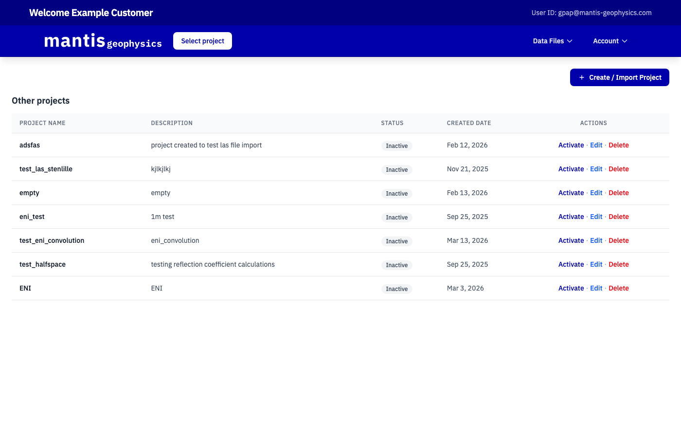
The projects list shows all of your projects. Each row displays the project name, description, status, creation date, and available actions:
- Activate — loads the project into memory and makes it the active project for all tools
- Edit — rename or update the project description
- Delete — permanently removes the project and all associated data
The currently active project appears at the top of the list under Current project with a green Active badge. Only one project can be active at a time.
Creating a project
Click + Create / Import Project to open the project creation page.
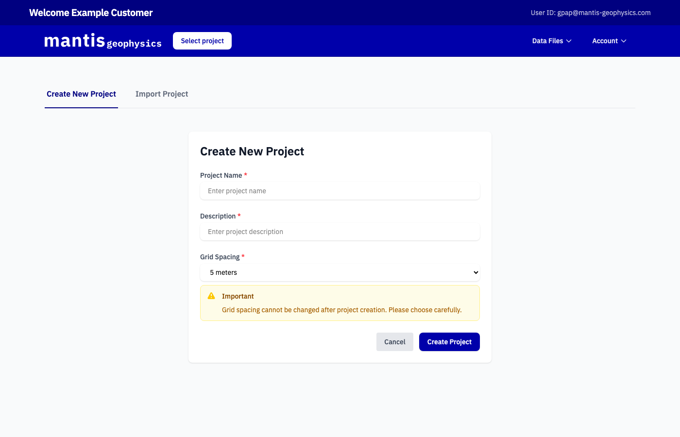
Two options are available via the tabs at the top:
Create New Project
Fill in the required fields:
| Field | Description |
|---|---|
| Project Name | A short, memorable name for the project |
| Description | A brief description of the model or survey |
| Grid Spacing | The spatial grid spacing used for finite-difference simulations |
Warning
Grid spacing cannot be changed after a project is created. Choose carefully based on the resolution required for your forward modelling.
Click Create Project to create the project. You can then activate it from the projects list.
Import Project
Use the Import Project tab to create a project from a .csv file. This is useful when you have an interpreted blocky well log and want to populate the project layers automatically.
The expected CSV format is a table with the following columns:
| Column | Unit | Required |
|---|---|---|
top_depth |
metres | Yes |
vp |
km/s | Yes |
vs |
km/s | Yes |
rho |
g/cm³ | Yes |
formation_name |
— | No |
Example:
| top_depth | vp | vs | rho | formation_name |
|---|---|---|---|---|
| 0 | 3.5 | 1.7 | 2.5 | Overburden |
| 1100 | 6.0 | 2.8 | 2.6 | Eau Clair Shale |
| 1500 | 4.7 | 2.6 | 2.5 | Mt. Simon Sandstone |
| 1700 | 4.5 | 2.4 | 2.45 | Mt. Simon Sandstone |
A sample file for the Decatur CO₂ injection site is available here.
Project overview
Click on a project name in the projects list to open its Overview page.
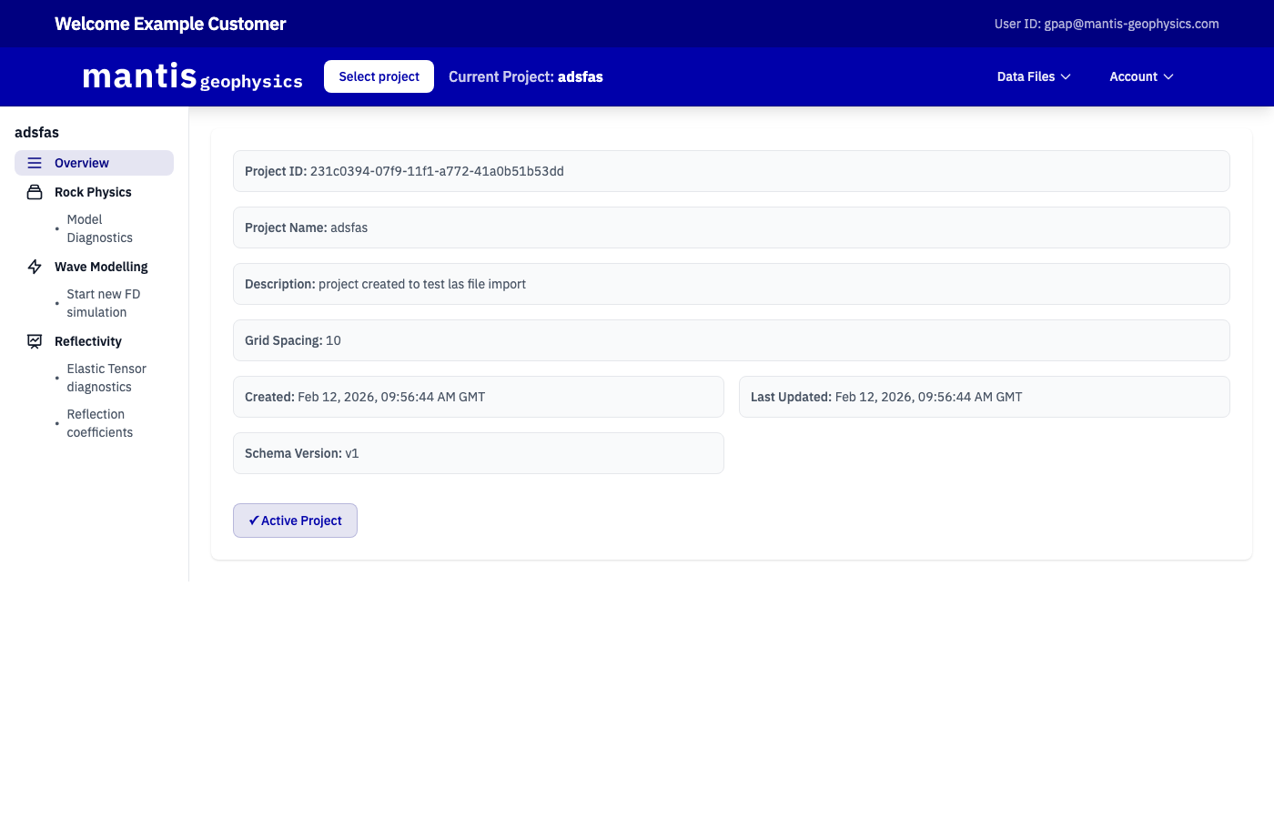
The overview shows the project metadata: name, description, grid spacing, creation and last-updated timestamps.
The left sidebar provides navigation to all tools available for this project:
| Section | Sub-page | Description |
|---|---|---|
| Overview | — | Project metadata |
| Rock Physics | Model Diagnostics | Configure layer properties and run rock physics models |
| Wave Modelling | Start new FD simulation | Launch a 2D finite-difference seismic simulation |
| Reflectivity | Elastic Tensor diagnostics | Analyse elastic tensors for any layer |
| Reflectivity | Reflection coefficients | Calculate halfspace reflection coefficients at layer interfaces |
If this is the active project, an ✓ Active Project badge is shown. Click View FD Simulations to jump directly to the wave model jobs list for this project.
Rock Physics — Model Diagnostics
Navigate to Rock Physics → Model Diagnostics in the sidebar.
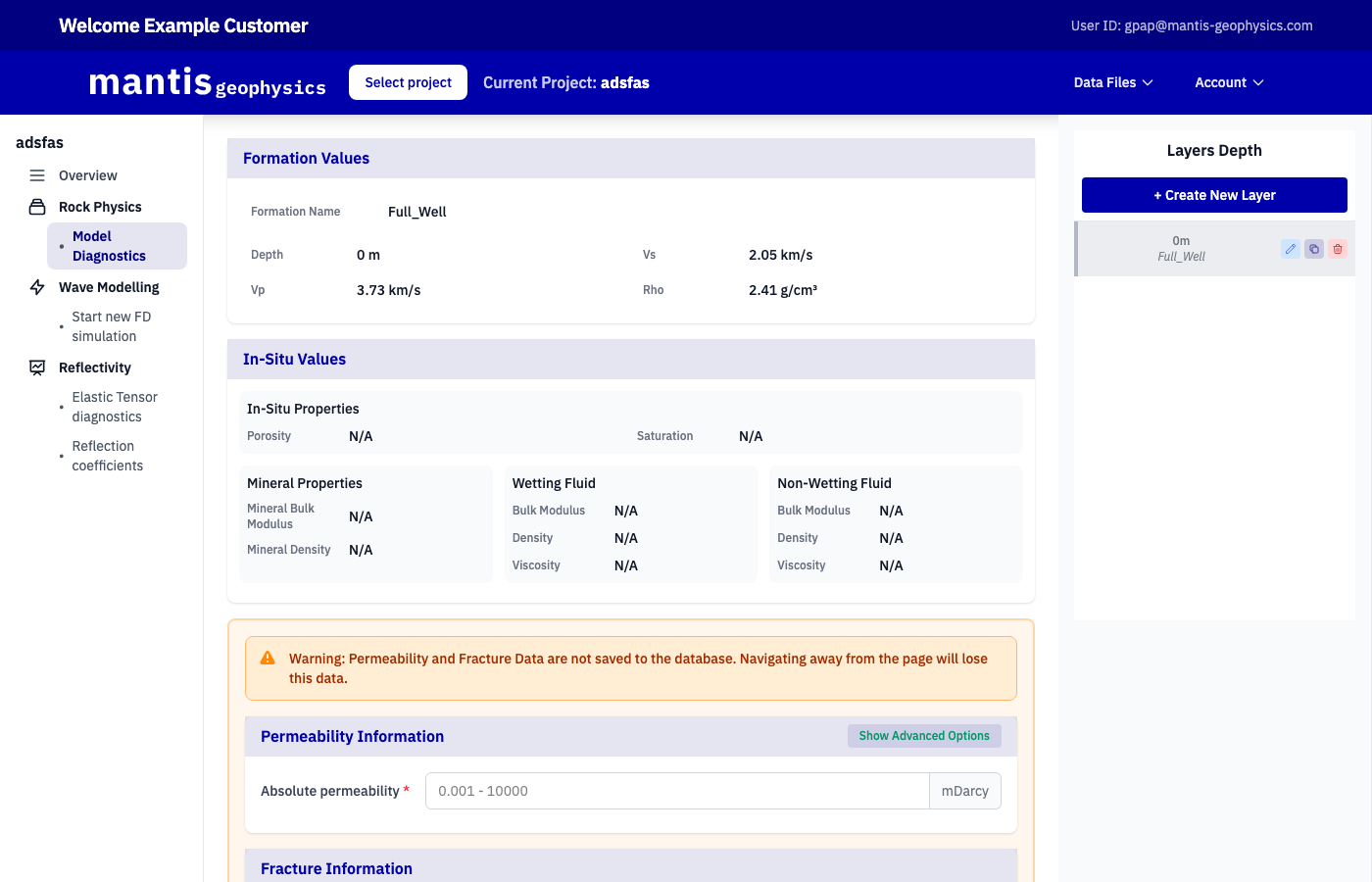
The Layers Depth panel on the right lists all layers in the project. Click + Create New Layer to add a layer, or select an existing layer to view and edit it.
Formation values
The Formation Values section shows the background elastic properties of the selected layer:
| Property | Description |
|---|---|
| Formation Name | Geological formation label |
| Depth | Top depth of the layer (m) |
| Vp | P-wave velocity (km/s) |
| Vs | S-wave velocity (km/s) |
| Rho | Density (g/cm³) |
These values are the background (in-situ) medium properties and are set when the layer is created.
In-situ values
The In-Situ Values section is used to define the pore fluid state of the layer for rock physics modelling. Fill in:
- Porosity and Saturation (in-situ conditions)
- Mineral Properties — Mineral Bulk Modulus and Mineral Density
- Wetting Fluid — Bulk Modulus, Density, and Viscosity
- Non-Wetting Fluid — Bulk Modulus, Density, and Viscosity
The dry frame modulus is back-calculated using the inverse Gassmann relation from the in-situ elastic properties and fluid state.
Permeability & fracture information
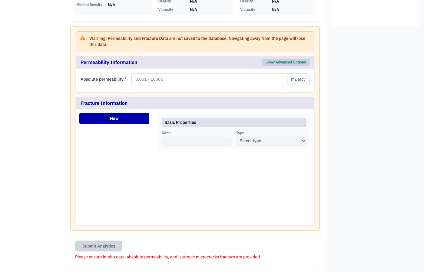
Warning
Permeability and fracture data are not saved to the database. Navigating away from the page will discard this data.
Permeability Information takes the absolute permeability of the layer in mDarcy. Click Show Advanced Options for additional permeability parameters.
Fracture Information allows you to define one or more fracture sets for the layer. Click New to add a fracture set and specify:
- Name — a label for the fracture set
- Type — the fracture model (e.g. isotropic microcracks using the Hudson 1980 model)
Fractures are created with faces normal to the vertical axis (VTI symmetry) by default. The Hudson model returns Thomsen anisotropy parameters for the fractured medium.
When all required in-situ data, permeability, and fracture information are provided, click Submit Analytics to run the rock physics model and store the results for use in reflectivity and wave modelling.
Note
The attenuation model uses the Standard Linear Solid (SLS) formulation, which gives frequency-dependent (peak intrinsic) attenuation rather than constant-Q attenuation. Causality is respected.
Reflectivity — Elastic Tensor diagnostics
Navigate to Reflectivity → Elastic Tensor diagnostics in the sidebar.
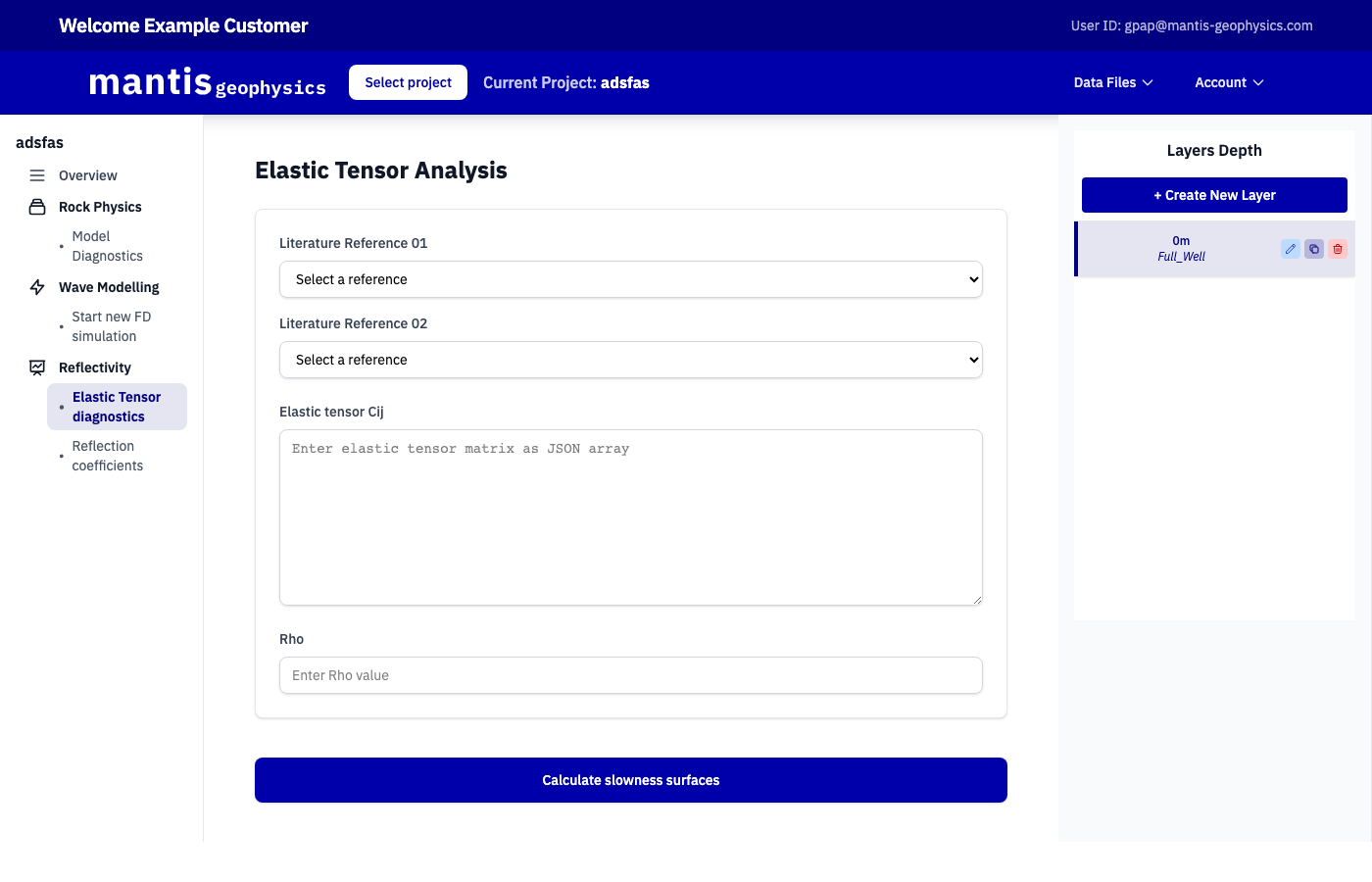
This tool allows you to analyse the full elastic tensor \(C_{ij}\) for any layer. Use it to inspect and validate the anisotropic elastic properties of a modelled layer.
| Input | Description |
|---|---|
| Literature Reference 01 / 02 | Optional references for the elastic tensor values |
| Elastic tensor C\(_{ij}\) | The 6×6 Voigt stiffness matrix entered as a JSON array |
| Rho | Density of the medium (g/cm³) |
Click Calculate slowness surfaces to compute and visualise the phase velocity slowness surfaces for the specified tensor.
Reflectivity — Reflection coefficients
Navigate to Reflectivity → Reflection coefficients in the sidebar.
Note
At least two layers must be configured in the project before reflection coefficients can be calculated. This page will display an "Insufficient Layers" message if fewer than two layers exist.
This tool calculates halfspace reflection and transmission coefficients at any layer interface in the project. By convention, layers are identified by their top depth; the selected layer is treated as the lower halfspace of a two-layer model.
Viscoelastic (frequency-dependent) media
If a layer is viscoelastic (attenuating), reflection coefficients are frequency-dependent. The calculation is performed at three frequency regimes: low (\(\approx 0.1\,f_0\)), central (\(f_0\)), and high (\(\approx 10\,f_0\)), where \(f_0\) is the dominant frequency of the assumed plane-wave source.
Anisotropic media
If a layer is anisotropic (fractured), the fractures are modelled using the Hudson model with VTI symmetry by default. Fracture tilt and azimuth sliders allow you to rotate the fracture orientation:
- Tilt = 0° — vertical fractures (VTI symmetry)
- Azimuth = 90° — fractures aligned along the x-axis (HTI symmetry)
A further rotation in the azimuthal plane is available when the tilt differs from 0°.
Wave Modelling — Start new FD simulation
Navigate to Wave Modelling → Start new FD simulation in the sidebar.
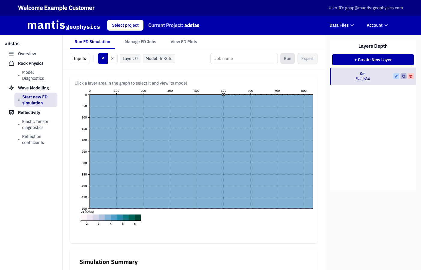
Selecting a model for each layer
The Available Models panel lists all rock physics scenarios that have been submitted via Model Diagnostics. Select the scenario you want to use for each layer in the project. Only layers for which analytics have been submitted will appear.
Wave model input parameters
Configure the simulation parameters under Wave Model Input Parameters:
| Parameter | Description |
|---|---|
| Offset VSP arrays to record during simulation | Number of offset VSP receiver arrays (1–20) |
| Source time function | Wavelet shape: Ricker (default) or User Input |
| Peak frequency of the source | Dominant frequency of the source wavelet in Hz (20–80 Hz) |
Simulation summary
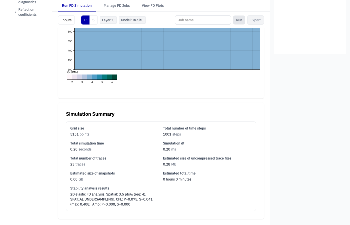
Before launching, review the Simulation Summary which shows the estimated computational cost:
| Field | Description |
|---|---|
| Grid size | Total number of spatial grid points |
| Total number of time steps | Time-domain steps to be computed |
| Total simulation time | Physical duration of the simulation (seconds) |
| Simulation dt | Time step size (ms) |
| Total number of traces | Number of seismic traces to be recorded |
| Estimated size of uncompressed trace files | Approximate output file size (MB) |
| Estimated size of snapshots | Approximate wavefield snapshot storage (GB) |
| Estimated total time | Predicted wall-clock run time |
| Stability analysis results | CFL and amplitude stability conditions |
Enter a descriptive job name, then click Start Job to submit the simulation. Click Expert Mode for additional low-level solver parameters.
Note
Simulation run time depends on the project size and grid spacing and may range from a few minutes to several hours.
Wave Modelling — Managing simulations
To view existing simulations, click View FD Simulations from the project Overview, or navigate to the wave model jobs page directly.
The Wave Model Jobs table lists all simulations for the active project with their name, job ID, status, status message, and submission time. Click Refresh to update the list.
Available actions per job (shown in the Actions column once jobs are present):
- Download — download seismograms, wavefield snapshots, and a parameter log
- Stop — cancel a running simulation
- Delete — permanently remove the simulation record
Warning
Simulation records are retained for a grace period of 30 days after your contract expires, after which they are permanently deleted without the possibility of recovery.